The HSOM class

This tutorial will help you understand the core of HySOM, the HSOM class. You will learn the fundamental methods for training and exploring a trained SOM. To demonstrate its functionality, we will use a sample dataset included with HySOM. More details on the HSOM class can be found in the API reference

import numpy as np
from hysom import HSOM 
from hysom.utils.datasets import get_labeled_loops
import matplotlib.pyplot as plt

Get sample data

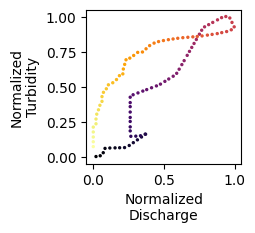
loops, labels = get_labeled_loops()

print(f"The sample data consists of {len(loops)} labeled loops")
print(f"Each loop is a matrix of shape: {loops[0].shape}")
print("Example: ")
sample_loop = loops[np.random.choice(len(loops))]
plt.figure(figsize=(2,2))
_ = plt.scatter(sample_loop[:,0],sample_loop[:,1], s = 2, cmap = "inferno", c = range(len(sample_loop)))
plt.xlabel("Normalized\nDischarge")
plt.ylabel("Normalized\nTurbidity")

The sample data consists of 340 labeled loops
Each loop is a matrix of shape: (100, 2)
Example: 

Text(0, 0.5, 'Normalized\nTurbidity')

Training a SOM

Creating a new SOM instance requires three mandatory arguments to define the SOM’s lattice dimensions and the input data dimensions: width, heightand input_dim. Currently, only 2D sequences are supported, meaning the input_dim should follow the format: (sequence_length,2).
Additionally, you can specify an optional random_seed to ensure reproducibility

mysom = HSOM(width=5, height=5, input_dim = (100,2), random_seed=1234567)

Once instantiated, the train method can be called with two mandatory arguments: data, which is a sequence of training loops, and epochs, which defines the number of training iterations (each loop is fed to the map once per epoch). Several optional arguments provide full control over the training process, including distance_function (defaults to Dynamic Time Warping), neighborhood_function (defaults to Gaussian), [initial/final]_learning_rate, and more (see the API reference).
In this tutorial, we will only include track_errors to record the history of the quantization and topographic errors during training and verbose to get reports of the training process in the console.

epochs = 5
mysom.train(data= loops, epochs = epochs, track_errors=True, verbose = 4)

============================================================
Epoch: 1/5 - Quant. Error: 0.91 - Topo. Error: 0.65
[85/340] 25%
[170/340] 50%
[255/340] 75%
[340/340] 100%
============================================================
Epoch: 2/5 - Quant. Error: 1.43 - Topo. Error: 0.0
[85/340] 25%
[170/340] 50%
[255/340] 75%
[340/340] 100%
============================================================
Epoch: 3/5 - Quant. Error: 1.25 - Topo. Error: 0.0
[85/340] 25%
[170/340] 50%
[255/340] 75%
[340/340] 100%
============================================================
Epoch: 4/5 - Quant. Error: 1.02 - Topo. Error: 0.0
[85/340] 25%
[170/340] 50%
[255/340] 75%
[340/340] 100%
============================================================
Epoch: 5/5 - Quant. Error: 0.91 - Topo. Error: 0.0
[85/340] 25%
[170/340] 50%
[255/340] 75%
[340/340] 100%
============================================================
Training Completed! - Quant. Error: 0.87 - Topo. Error: 0.0
============================================================

The trained prototypes (also called codebooks or weight vectors in the SOM jargon) can be extracted using get_prototypes()

trained_prototypes = mysom.get_prototypes()

print(f"Prototypes are {type(trained_prototypes)} of shape: {trained_prototypes.shape}")

Prototypes are <class 'numpy.ndarray'> of shape: (5, 5, 100, 2)

Visualize Prototypes

Checkout This tutorial to explore the visualization functions in detail

from hysom.utils.plots import plot_map

_ = plot_map(mysom.get_prototypes())

Inspecting Quantization and Topographic Errors

While quantization and topographic errors are displayed in the console after each epoch, the full history can be accessed using get_QE_history and get_TE_history. The QE and TE histories are useful to diagnose the training process

qe_iter_index, qe = mysom.get_QE_history()
te_iter_index, te  = mysom.get_TE_history()

Let’s plot them!

fig, (ax_qe, ax_te) = plt.subplots(2,1, figsize = (10,4), sharex=True)

# Plot topographic and quantization errors
ax_qe.plot(qe_iter_index, qe)
ax_te.plot(te_iter_index, te)
ax_qe.set_ylabel("Quantizaiton Error")
ax_te.set_xlabel("Iteration")
ax_te.set_ylabel("Topographic Error")

# Mark epochs
iterations_per_epoch = len(loops)
idx = 0
for i in range(epochs+1):
    ax_qe.axvline(idx, color = "grey", linestyle  = "--", alpha = 0.5)
    ax_te.axvline(idx, color = "grey", linestyle  = "--", alpha = 0.5)
    idx += iterations_per_epoch

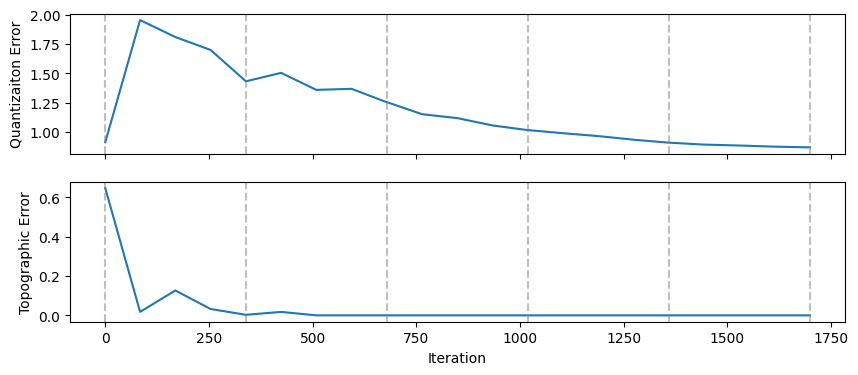
Note that TE and QE are not computed after each iteration, as doing so would be computationally expensive. You can control how often errors are computed using the errors_sampling_rate argument of the train method. By default, this value is set to 4, meaning errors are computed four times per epoch, plus an initial computation at the very beginning.

qe_iter_index[:5]

(0, 84, 169, 254, 339)

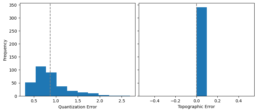
If you need to compute QE and TE for an arbitrary dataset using the final trained SOM, you can use the quantization_error and topographic_error methods (we’ll use the same training data but other datasets, not used during training, can be used as well). These methods return the TE and QE for each sample in the provided dataset

QE_final = mysom.quantization_error(loops)
TE_final = mysom.topographic_error(loops)

fig, (axqe, axte) = plt.subplots(1,2, sharey=True, figsize = (10,4))
axqe.hist(QE_final)
axte.hist(TE_final)
axqe.axvline(np.mean(QE_final), linestyle= "--", color = "grey")
axte.axvline(np.mean(TE_final), linestyle= "--", color = "grey")
axqe.set_ylabel("Frequency")
axqe.set_xlabel("Quantization Error")
axte.set_xlabel("Topographic Error")
plt.subplots_adjust(wspace=0.03)

Classifying a new sample

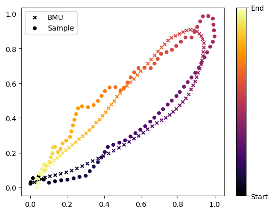
With a trined SOM, you can classify a sample using the get_BMU method.
See below how to efficiently classify multiple samples

sample_idx = np.random.randint(0, len(loops))
sample = loops[sample_idx]
BMU = mysom.get_BMU(sample)
print(BMU)

(2, 4)

get_BMU returns the coordinates of the Best Matching Unit following matrix notation (row, col). The associated prototype can be obtained using: get_prototypes()[BMU]

matching_prototype = mysom.get_prototypes()[BMU]

Let’s plot the sample and matching prototypes as trajectory plots

plt.figure()
plt.scatter(matching_prototype[:,0], matching_prototype[:,1], c = range(len(sample)), cmap = "inferno", s = 20, marker = "x", label = "BMU")
sc = plt.scatter(sample[:,0], sample[:,1], c = range(len(sample)), cmap = "inferno", s = 20, label = "Sample")

cb = plt.colorbar(sc)
cb.ax.set_yticks(ticks = [0, len(sample)], labels = ["Start", "End"])
plt.legend()

<matplotlib.legend.Legend at 0x1e9b47b3e00>

Classify multiple samples

Use the HSOM method classify to group samples according to their BMU:

classified_loops = mysom.classify(loops)

print("   BMU     # of loops")
for BMU, loops_list in classified_loops.items():
    print(f"{str(BMU):10s}    {len(loops_list)}")

   BMU     # of loops
(3, 2)        12
(2, 2)        26
(3, 1)        10
(2, 1)        9
(0, 4)        16
(0, 3)        11
(1, 3)        6
(1, 4)        12
(4, 0)        11
(4, 1)        15
(0, 2)        17
(0, 1)        8
(1, 0)        3
(1, 1)        15
(3, 0)        18
(2, 0)        18
(1, 2)        12
(3, 3)        14
(4, 3)        9
(3, 4)        9
(2, 3)        11
(2, 4)        19
(4, 2)        18
(4, 4)        21
(0, 0)        20

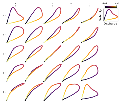
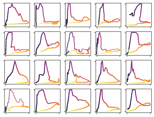
You can plot the loops associated to a BMU as follows:

selected_bmu = (0,0)

fig = plt.figure()
for i, loop in enumerate(classified_loops[selected_bmu]):
    ax = fig.add_subplot(4,5,i+1)
    ax.scatter(loop[:,0], loop[:,1], cmap= "inferno", s = 2, c = range(len(loop)))
    ax.tick_params(labelbottom = False, labelleft = False)

Compare them with the associated prototype:

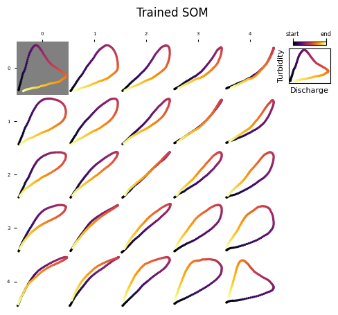
axs = plot_map(mysom.get_prototypes(), coordinates_style="matrix")
axs[selected_bmu].set_facecolor("gray")
axs[selected_bmu].figure.suptitle("Trained SOM")

Text(0.5, 0.98, 'Trained SOM')